How to auto-generate network diagrams based on Netbox

Undoubtedly, having appropriate and up-to-date documentation is one of the biggest challenges organisations face nowadays. Some organisations do manage to build some good documentation in the beginning. However, as time goes by new changes are made but the documentation never gets updated as other (revenue-generating) projects take priority leading to unuseful documentation.

So what do we do you may ask? The solution lies in treating the documentation in a similar fashion to the configuration of devices, that is, automating it.

Rather than updating diagrams every time a change is made to the network or a new data centre is built, we rely on the same Single Source Of Truth that our network provisioning automation does to generate the new documentation.

For this to work, of course, we need to have a Single Source Of Truth, to begin with. The idea behind this is to have a single point of control for the whole network, no more relying on excel spreadsheet for certain things, logging into devices for others and so on, but modelling all the config in a single place, and triggering all the automation based on this.

Everything has to be defined in the SSOT¹ and built based on it. There should not exist the option of bypassing the Source Of Truth. That way, you get to a point where you can even draw diagrams of your network at any time to have accurate documentation! For this example, I’m going to use Netbox as the single source of truth.

This post is going to be divided into two major areas, extracting the data from Netbox and building the diagram based on that data.

Extracting the data from the source of truth - Netbox

One of the key requirements for this to work is to have everything properly docummented in Netbox. This not only means having all the correct data in there but also having the proper metadata (data about the data). For instance, if we have no way to uniquely identify all our spine switches in a single DC, then we can’t really build a sane script to gather this information and make use of it.

A reasonable solution for this is to add the device_role ‘spine’ to every spine switch. This would allow us to do something like this:

In [275]: list(nb.dcim.devices.filter(role='spine', site='us-east'))
Out[275]: [spine1, spine2, spine3, spine4]

As you can see, given the role and site we managed to extract all spines in a given location. The same can be done to extract all the leaves:

In [276]: list(nb.dcim.devices.filter(role='leaf', site='us-east'))
Out[276]: [leaf1, leaf2, leaf3, leaf4, leaf5, leaf6, leaf7, leaf8]

Now, let’s first create a function to get all the connections from a device given it’s name and site. This will allow us to generate any type of diagram ranging from ad-hoc diagrams for specific leaves to building the entire leaf-spine fabric for a given DC.

def find_connections(nb, device, site):
    """
    Given a device, it finds all its connections and returns a dictionary
    with the mapping {'queried_device_interface': (connected_device_name, connected_device_interface)
    """
    interfaces = list(nb.dcim.interfaces.filter(device=device, site=site))
    result = {}
    for interface in interfaces:
        connected_device_interface = interface.connected_endpoint
        if connected_device_interface is not None:
            connected_device_name = interface.connected_endpoint.device
            result[f'{interface}'] = (connected_device_name, connected_device_interface)
    return result

This function will genererate the following data structure:

In [271]: find_connections(nb, 'spine1', 'us-east')
Out[271]: 
{'swp1': (leaf1, swp29),
 'swp2': (leaf2, swp29),
 'swp3': (leaf3, swp29),
 'swp4': (leaf4, swp29),
 'swp5': (leaf5, swp29),
 'swp6': (leaf6, swp29),
 'swp7': (leaf7, swp29),
 'swp8': (leaf8, swp29)}

Each key of the dictionary contains an interface in the queried device (‘spine1’) that has something connected to it. Each value contains a tuple where the first value is the far-end device name, and the second is the far-end interface name.

How about from the perspective of the leaf?

In [277]: find_connections(nb, 'leaf1', 'us-east')
Out[277]: 
{'swp29': (spine1, swp1),
 'swp30': (spine2, swp1),
 'swp31': (spine3, swp1),
 'swp32': (spine4, swp1)}

Building the diagram using Graphviz

When it comes to building the diagram there are three parts we need to understand:

graph TD;
	A[1-Netbox Data]--using python library-->B[2-Generate graph description in DOT language]--using Graphviz-->C[3-Generate diagram in PDF/PNG/SVG]

We already covered the general idea of the first step in the previous section, so let’s take a look at how to use the Python Graphviz library to generate the graph description in the DOT language format.

There are many tools out there, some easier to use and some more complex, for this example I’ve chosen ‘Graphviz’ as it seems to do the job reasonably well however, you don’t necessarily have to use this, the key idea from this post is to shift from the old mindset of maintaining network diagrams manually and move into the new world of Infrastructure as Code aka IaC.

First make sure you install the library:

pip install graphviz

Then, let’s generate the graph description in the DOT language:

diagram_name = 'US East Data Centre Diagram'

# Create a graph object - the output format is also selected here
dot = graphviz.Graph(engine='dot', format='pdf', node_attr={
    'shape': 'rectangle',
})

# Create all nodes (spine and leaf devices)
for spine in spines:
    dot.node(f'{spine}', ordering="out")
for leaf in leaves:
    dot.node(f'{leaf}', ordering="in")

# Create all edges (make the connections between spines and leaves)
for spine in spines:
    spine_connections = find_connections(nb, spine, 'us-east')
    for connection in spine_connections:
        leaf_name = spine_connections[connection][0]
        leaf_interface = spine_connections[connection][1]
        dot.edge(f'{spine}', f'{leaf_name}') # add label=f'{leaf_interface}' to include intf descr

# Print the graph description in the DOT language
print(dot.source)

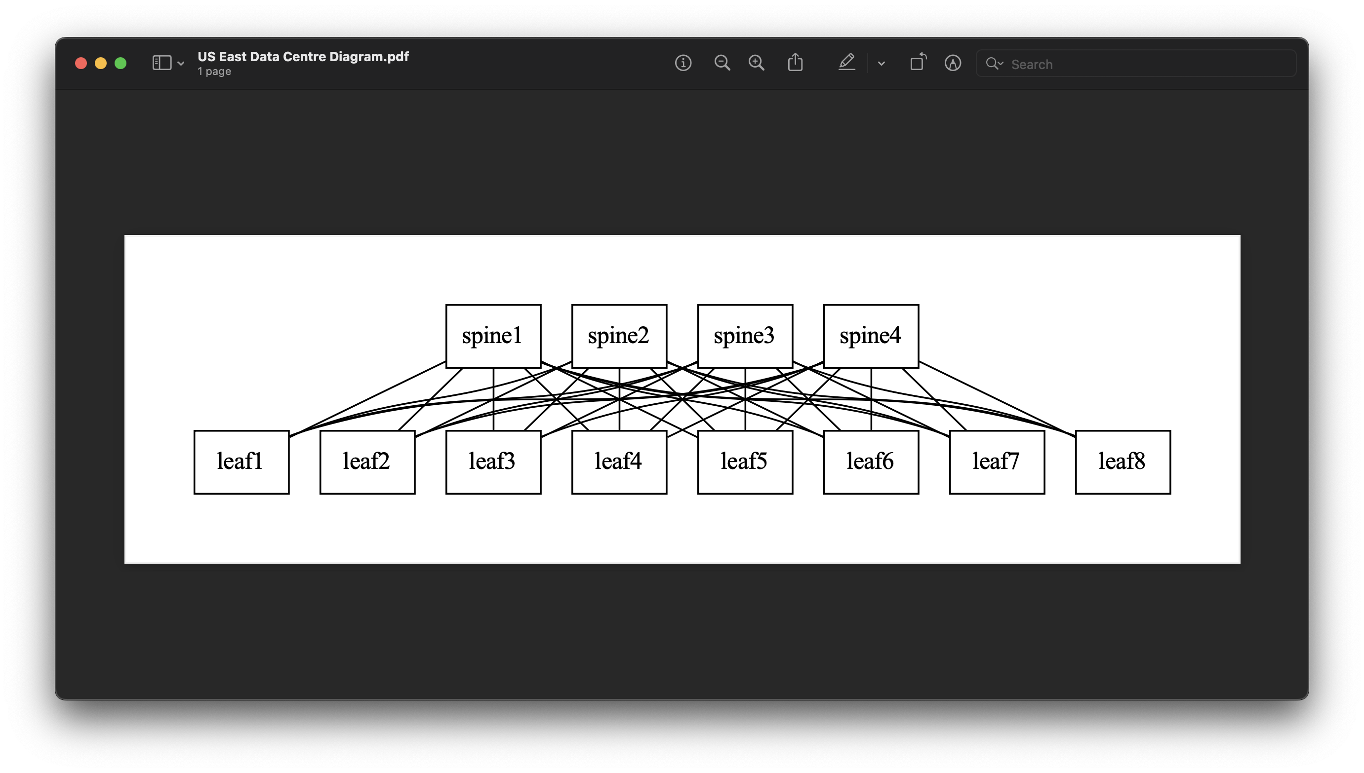
Lastly, let’s generate the actual diagram. This will create two files, a text file with the graph description in the DOT language and a pdf file with the graph diagram. The files will be save in the local directory, inside the “diagrams” folder.

dot.render(f'diagrams/{diagram_name}', view=True) # view=True means the pdf file will open automatically

You need to install the actual software Graphviz (different from the python library installed previously) in your local machine in order to be able to generate the diagrams. If you’re using a MAC you can run “brew install graphviz” or “apt-get install graphviz” for debian-based distros.

Here’s our diagram:

And here’s our graph description in the DOT language:

graph {
        node [shape=rectangle]
        spine1 [ordering=out]
        spine2 [ordering=out]
        spine3 [ordering=out]
        spine4 [ordering=out]
        leaf1 [ordering=in]
        leaf2 [ordering=in]
        leaf3 [ordering=in]
        leaf4 [ordering=in]
        leaf5 [ordering=in]
        leaf6 [ordering=in]
        leaf7 [ordering=in]
        leaf8 [ordering=in]
        spine1 -- leaf1
        spine1 -- leaf2
        spine1 -- leaf3
        spine1 -- leaf4
        spine1 -- leaf5
        spine1 -- leaf6
        spine1 -- leaf7
        spine1 -- leaf8
        spine2 -- leaf1
        spine2 -- leaf2
        spine2 -- leaf3
        spine2 -- leaf4
        spine2 -- leaf5
        spine2 -- leaf6
        spine2 -- leaf7
        spine2 -- leaf8
        spine3 -- leaf1
        spine3 -- leaf2
        spine3 -- leaf3
        spine3 -- leaf4
        spine3 -- leaf5
        spine3 -- leaf6
        spine3 -- leaf7
        spine3 -- leaf8
        spine4 -- leaf1
        spine4 -- leaf2
        spine4 -- leaf3
        spine4 -- leaf4
        spine4 -- leaf5
        spine4 -- leaf6
        spine4 -- leaf7
        spine4 -- leaf8
}

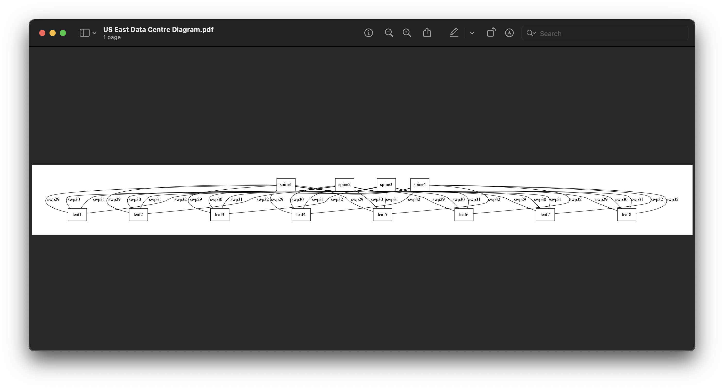
Let’s include the leaf interfaces:

dot.edge(f'{spine}', f'{leaf_name}', label=f'{leaf_interface}')

Diagram:

As you can see, it doesn’t look as nice but the is a good thing about it: the diagram is in PDF format, which means we can ctr-f for whatever we’re looking for. That’s useful, especially when we have very large diagrams:

Full script

import graphviz
import pynetbox

NETBOX_URL = 'http://localhost:8000'
TOKEN = '0123456789abcdef0123456789abcdef01234567'
nb = pynetbox.api(url=NETBOX_URL, token=TOKEN)

def find_connections(nb, device, site):
    """
    Given a device, it finds all its connections and returns a dictionary
    with the mapping {'queried_device_interface': (connected_device_name, connected_device_interface)
    """
    interfaces = list(nb.dcim.interfaces.filter(device=device, site=site))
    result = {}
    for interface in interfaces:
        connected_device_interface = interface.connected_endpoint
        if connected_device_interface is not None:
            connected_device_name = interface.connected_endpoint.device
            result[f'{interface}'] = (connected_device_name, connected_device_interface)
    return result


if __name__ == '__main__':
    diagram_name = 'US East Data Centre Diagram'
    leaves = list(nb.dcim.devices.filter(role='leaf', site='us-east'))
    spines = list(nb.dcim.devices.filter(role='spine', site='us-east'))

    # Create a graph object - the output format is also selected here
    dot = graphviz.Graph(engine='dot', format='pdf', node_attr={
        'shape': 'rectangle',
    })

    # Create all nodes (spine and leaf devices)
    for spine in spines:
        dot.node(f'{spine}', ordering="out")
    for leaf in leaves:
        dot.node(f'{leaf}', ordering="in")

    # Create all edges (make the connections between spines and leaves)
    for spine in spines:
        spine_connections = find_connections(nb, spine, 'us-east')
        for connection in spine_connections:
            leaf_name = spine_connections[connection][0]
            leaf_interface = spine_connections[connection][1]
            dot.edge(f'{spine}', f'{leaf_name}', label=f'{leaf_interface}')
            # dot.edge(f'{spine}', f'{leaf_name}')
            
    # Print the graph description in DOT language
    print(dot.source)
    dot.render(f'diagrams/{diagram_name}', view=True)

Conclusion

We’ve just discussed the tip of the iceberg in regards to this new world of Infastructure as Code and more specifically Code as documentation. Ultimately, you’d need to define the scope of your diagrams, perhaps drawing a whole DC may render the diagram unreadable (although using ctl-f may be good enough for you) and you’d want instead per-pod diagrams or any other thing you can think of.

I’ve tried to follow a modular approach whereby you can replace any of the components with any other tool but still follow the same system:

Base everything on a Single Source Of Truth
Extract the data from it
Generate a diagram based on that data using your tool of choice

Extracting the data from the source of truth - Netbox

Building the diagram using Graphviz

Full script

Conclusion

Further Reading